Introduction
This vignette demonstrates a full ezTrack workflow: importing tracking data with non-standard column names, cleaning and standardizing it, converting it to a spatial object, generating summary tables, visualizing fix rates and latitude over time, and plotting tracks and home ranges on an interactive map.
1. Import and format tracking data
We pass a dataset of GPS-tagged migratory shorebirds to
ez_track(). If column names aren’t provided,
ez_track() will automatically attempt to guess which
columns correspond to ID, timestamp, longitude, and latitude.
data(godwit_tracks)
head(godwit_tracks)
#>      individual.local.identifier           timestamp location.long location.lat
#> 3935                     animal1 2024-12-31 16:00:00     -15.84644     16.33822
#> 3936                     animal1 2024-12-31 20:00:00     -15.82790     16.38281
#> 3937                     animal1 2024-12-31 22:00:00     -15.82829     16.38226
#> 3938                     animal1 2025-01-01 00:00:00     -15.82715     16.38327
#> 3939                     animal1 2025-01-01 04:00:00     -15.82761     16.38304
#> 3940                     animal1 2025-01-01 10:00:00     -15.84629     16.32770

tracks <- ez_track(
  data = godwit_tracks
)
#> Detected columns - id: individual.local.identifier, timestamp: timestamp, x: location.long, y: location.lat
#> Removed 852 row(s) with missing or duplicate values.
If automatic column guessing fails or guesses incorrectly, you can manually specify which columns represent the ID, timestamp, longitude, and latitude.
tracks_manual <- ez_track(
  data = godwit_tracks,
  id_col = 'individual.local.identifier',
  time_col = 'timestamp',
  x_col = 'location.long',
  y_col = 'location.lat',
)
#> Detected columns - id: individual.local.identifier, timestamp: timestamp, x: location.long, y: location.lat
#> Removed 852 row(s) with missing or duplicate values.
You can also subsample the dataset using the subsample()
argument, which limits the number of location fixes per time unit. Use a
simple string format such as “1 per hour” or “2 per day” to control the
sampling frequency.
tracks_subsampled <- ez_track(
  data = godwit_tracks,
  subsample = "2 per hour"
)
#> Detected columns - id: individual.local.identifier, timestamp: timestamp, x: location.long, y: location.lat
#> Removed 852 row(s) with missing or duplicate values.
#> Subsampled to 2 fix(es) per hour
2. Tracking data summary reports
Summary reports can be computed for each individual using
ez_summary(). For easy use in reports or presentations,
HTML reports can be generated using report = TRUE.
Summaries can also be filtered by date using the start_date
and end_date arguments.
The following summary statistics are returned for each unique id:
- n_fixes: Number of location records
- first_location: Timestamp of the first recorded location
- last_location: Timestamp of the last recorded location
- tracking_duration_days: Duration between first and last fix (in
days)
- fixes_per_day: Average number of fixes per day
- median_interval_hours: Median interval between fixes (in
hours)
- max_time_gap_days: Longest time gap between consecutive fixes (in
days)
- distance_km: Total distance traveled (in kilometers), calculated
using the Haversine formula
- avg_speed_kmh: Average speed (km/h), computed as distance divided by tracking duration in hours
summary_table <- ez_summary(tracks)
summary_table
#>        id n_fixes      first_location       last_location
#> 1 animal1    1095 2024-12-31 16:00:00 2025-04-25 14:00:00
#> 2 animal2    1153 2024-12-31 16:00:00 2025-04-27 22:00:00
#> 3 animal3    1022 2024-12-31 16:00:00 2025-04-23 16:00:00
#> 4 animal4     214 2024-12-31 16:00:00 2025-04-27 16:00:00
#> 5 animal5     223 2024-12-31 16:00:00 2025-04-27 16:00:00
#> 6 animal6     551 2024-12-31 16:00:00 2025-04-27 16:00:00
#>   tracking_duration_days fixes_per_day median_interval_hours max_time_gap_days
#> 1                 114.92          9.53                     2              0.33
#> 2                 117.25          9.83                     2              1.00
#> 3                 113.00          9.04                     2              1.00
#> 4                 117.00          1.83                     6             10.00
#> 5                 117.00          1.91                     6             13.38
#> 6                 117.00          4.71                     4              1.00
#>   distance_km avg_speed_kmh
#> 1     5649.19          2.05
#> 2     5495.39          1.95
#> 3     6370.80          2.35
#> 4     2414.07          0.86
#> 5     2372.16          0.84
#> 6     5438.92          1.94
3. Visualize latitude over time
ez_latitude_plot() can be used to visualize latitudinal
movement (north-south) over time for each tracked animal.
ez_latitude_plot(tracks)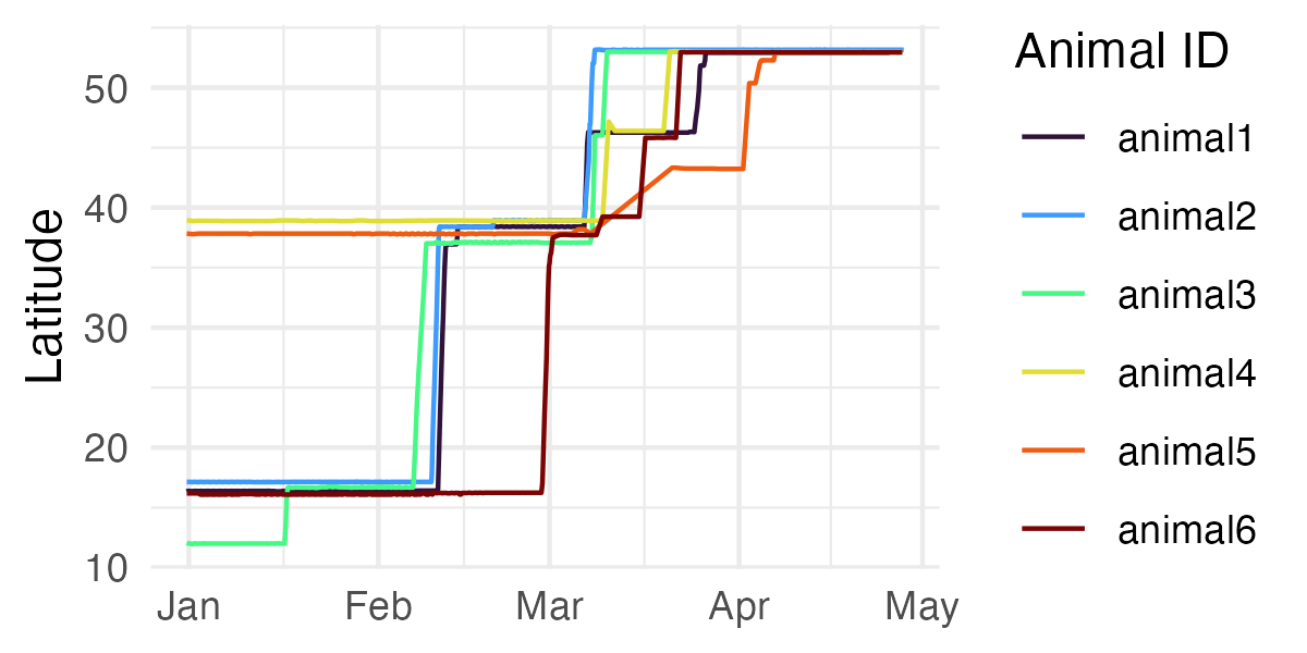
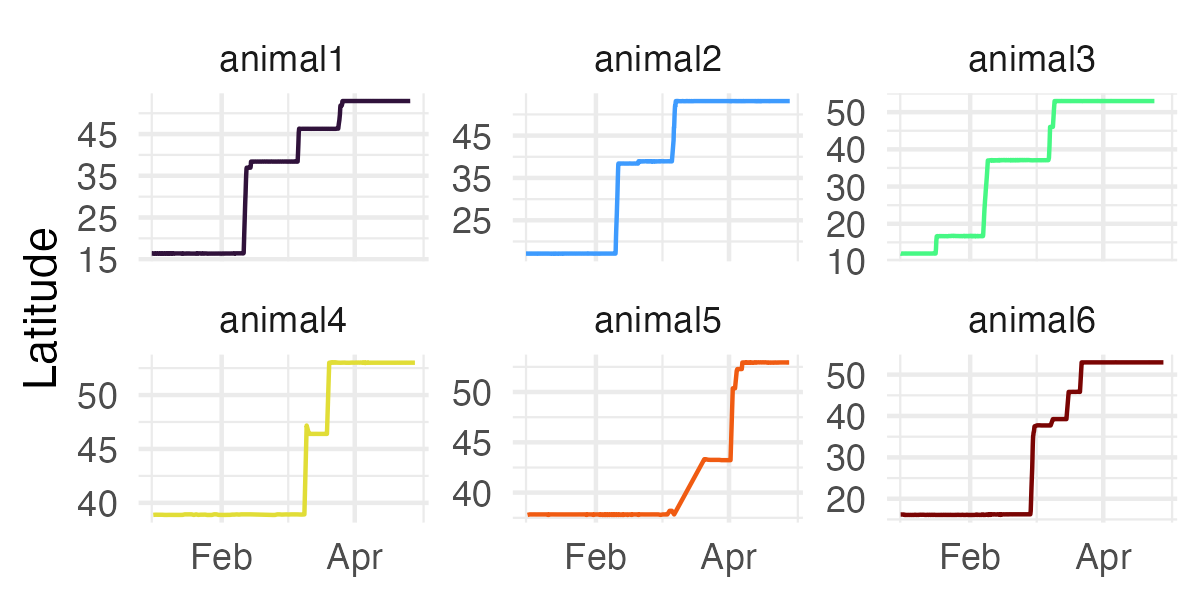
The plot supports:
Optional faceting by individual
Date axis customization
Date range filtering
ggplot2parameters for further customization.
ez_latitude_plot(
  tracks,
  facet = TRUE,
  start_date = "2025-01-01",
  end_date = "2025-04-28",
  date_breaks = "2 months",
  date_format = "%b"
)
4. Visualize fix rate over time
ez_fix_rate_plot() can be used to visualize fix rates
over time for each tracked animal, using a tick mark to represent each
location fix.
ez_fix_rate_plot(tracks)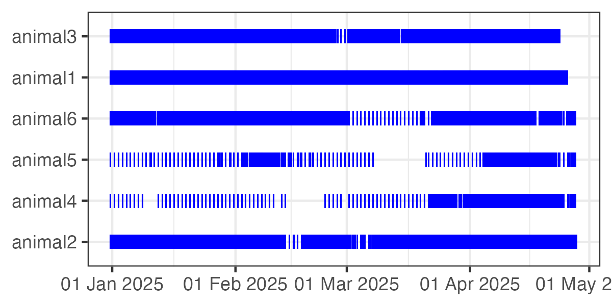
The plot supports:
Date axis customization
Date range filtering
ggplot2parameters for further customization.
5. Map tracks and home ranges
We can display tracks using an interactive Leaflet map with
ez_map() with a simple command.
ez_map(tracks)As well as with date range filters and a variety of style arguments.
ez_map(tracks,
  start_date = "2025-04-10",
  end_date = "2025-04-28",
  point_color = "timestamp",
  point_size = 2,
  path_opacity = 0.3)
6. Estimate home ranges
Individual or population-level Minimum Convex Polygons (MCP) or
Kernel Density Estimate (KDE) home ranges can be created with
ez_home_range().
home_ranges_mcp <- ez_home_range(tracks, method = 'mcp', level = 95, start_date = '2025-04-12')
#> Registered S3 methods overwritten by 'adehabitatMA':
#>   method                       from
#>   print.SpatialPixelsDataFrame sp
#>   print.SpatialPixels          sp
The result is an sf object containing one home range
polygon per tracked individual or population (if
population = TRUE).
Home ranges can be visualized with ez_map.
ez_map(home_ranges = home_ranges_mcp)Home ranges can also be mapped alongside tracking data. In this example, we use the start_date argument to ensure the tracking data aligns temporally with the home range period.
ez_map(tracks, home_ranges = home_ranges_mcp, start_date = '2025-04-12')